Week 11: Critical Thinking & Causal Inference – Endogeneity & Instrumental Variables (IV)

(Completed version)

This week is about a very common real‑world situation:

We want the effect of education on earnings, but we can't run a perfect experiment and we can't observe all the things that make some people both study more and earn more.

Ordinary least squares (OLS) then mixes up:

• the true causal effect of schooling on earnings, and

• the effect of unobserved factors like ability, motivation, or family background.

Instrumental variables (IV) give us a clever workaround. Instead of trying to perfectly measure all confounders, we look for a variable that nudges education up or down for reasons unrelated to those confounders.

In this lecture and lab we’ll use the classic example:

• Outcome: earnings

• Treatment: years of education

• Instrument: distance to the nearest college when you were a teenager

---

Learning goals

By the end of this week you should be able to:

• Explain, in words and pictures, why OLS can be biased when important confounders are unobserved.

• State and interpret the three core IV assumptions:

  • Relevance (the instrument actually moves the treatment),

  • Independence (as good as randomly assigned, conditional on controls),

  • Exclusion restriction (it affects the outcome only through the treatment).

• Read and explain an IV DAG using the education–earnings example.

• Describe the intuition behind two‑stage least squares (2SLS):

  • “First stage”: use the instrument to isolate the part of education that is as‑good‑as‑random.

  • “Second stage”: use only that part to estimate the causal effect on earnings.

---

1. Motivation: education and earnings

We care about the causal question:

If a person gets one extra year of schooling, how much do their earnings change on average?

Let

• $X$ = years of education
• $Y$ = earnings (e.g. log wages)
• $U$ = “everything else” that affects both $X$ and $Y$
  • e.g. ability, grit, family support, neighborhood, school quality, etc.

---

If we run a simple OLS regression $$ Y = \beta_0 + \beta_1 X + \varepsilon, $$ the slope $\beta_1$ will usually be too big or too small, because $X$ is positively or negatively related to $U$.

• Students with high ability / strong families might both study more and earn more → OLS overstates the causal effect.
• In some settings, people who stay longer in school might be those with fewer good outside options → OLS could understate the effect.

---

The key problem is:

We cannot see $U$, but $U$ affects both $X$ and $Y$.
This is the classic endogeneity / omitted variable bias problem.

---

Recap: Omitted Variable Bias (OVB) and the “ideal fix”

From the OVB lecture, you already know the basic story:

• If there is a variable that affects both education and earnings and we observe it, the fix is simple: include it as a control.

In an ideal world our wage equation would be

$$ \text{wage} = \beta_0 + \beta_1 \text{educ} + \beta_2 \text{ability} + u. $$

---

If we observed “true ability” we would just put it in the regression and OLS would not be biased by ability.

But in reality, things like true ability, motivation, family background are often

• hard to measure well, or
• completely unobserved.

Then they get absorbed into the error term, and since ability is correlated with education, we get

$$ \text{Corr}(\text{educ}, \varepsilon) \neq 0, $$

which is exactly endogeneity (a regressor correlated with the error).

So you can think of “unobserved OVB” as one of the main ways endogeneity shows up.

Takeaway 💡

• If we could measure ability well, the OVB lecture already told us what to do:
  just add it as a control and we’re fine.

• But for things like true ability or family background, we can’t measure them well.
  -> That’s exactly when OLS breaks, and we need a different trick — instrumental variables.

---

2. IV example and directed acyclic graph (DAG): distance to college

To deal with unobserved confounders, we look for an instrument $Z$.

In our example, a natural candidate is:

• $Z$: distance to the nearest college when the individual was a teenager

Intuition:

• If you grow up closer to a college, it's cheaper and easier to attend.
• So $Z$ should push education $X$ up or down, even for people who are otherwise similar.
• But, after controlling for broad region, living a bit closer or farther from a college should not directly change your earnings except through education.

---

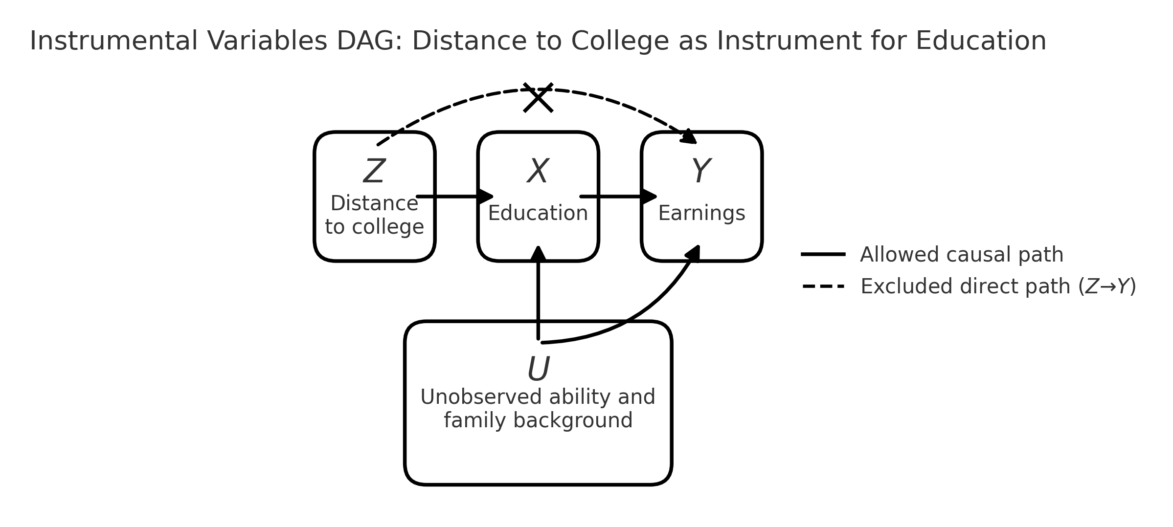
We will think in terms of four variables:

• $Z$: distance to college (instrument)
• $X$: education (endogenous treatment)
• $Y$: earnings (outcome)
• $U$: unobserved ability and family background (confounders)

The DAG below summarizes this story graphically.

• Solid arrows = allowed causal paths.
• Dashed arrow = “forbidden” direct effect that IV rules out (and the X on it reminds us of that).

---

3. IV assumptions in the DAG (with intuition)

From the DAG, we can read off three key assumptions. You should be able to explain each one in words.

3.1. Relevance: $Z$ really moves $X$

• Graphically: solid arrow $Z \to X$.
• People who grow up closer to a college are more likely to get more education.

---

3.2 Independence: $Z$ is “as‑good‑as‑random” w.r.t. $U$

• Graphically: no arrow between $Z$ and $U$.
• In words: conditional on simple controls (region, urban/rural, etc.), distance to college is not systematically related to unobserved ability or family background.

This is a research design judgment call: we argue that, after controls, families did not choose location in a way that’s tightly tied to their child’s unobserved ability.

---

3.3 Exclusion restriction: $Z$ affects $Y$ only through $X$

• Graphically: the dashed arrow $Z \to Y$ is crossed out.
• Distance to college has no direct effect on earnings except through its effect on education.

This rules out channels like “local wages are higher near colleges, even for equally educated workers” or “job networks from growing up near a campus, regardless of whether you attend”. If those effects are large, the instrument is not valid.

---

4. Two-stage least squares (2SLS) – intuition first

IV/2SLS is basically a two‑step filtering process:

1. Step 1: isolate the part of $X$ that comes from the instrument.
   We use $Z$ (and controls $W$) to predict education: $$ X_i = \pi_0 + \pi_1 Z_i + \pi_2 W_i + v_i. $$ The fitted values $\hat X_i$ are the part of education that is “explained by” distance to college and the controls.
   Intuition: this is the as‑good‑as‑random variation in schooling.

2. Step 2: see how outcomes move with this “clean” part of $X$.
   We then regress earnings on the predicted education: $$ Y_i = \beta_0 + \beta_1 \hat X_i + \beta_2 W_i + \varepsilon_i. $$ Now $\beta_1$ tells us: “If schooling goes up for reasons only related to $Z$ (and not $U$), how much do earnings change?”

Caution: In code, don’t literally run two separate OLS regressions and treat the fitted values as real data—always use an IV/2SLS command, otherwise the standard errors will be wrong.

---

5. OLS vs IV in a simple simulation (ability / family background story)

In this section, we build a toy world where we know the true effect of education on wages, and we deliberately introduce ability/family background as an omitted variable that creates upward bias in OLS.

---

5.1 Data-generating story

Each individual has:

• ability: unobserved ability / family background
• z: an instrument (e.g. "grew up near a college"), taking values 0 or 1
• educ: years of schooling
• wage: log wage

---

We assume:

1. Education decision

$$ \text{educ}_i = 12 + 2 z_i + 1.0 \cdot \text{ability}_i + u_i $$

• Baseline schooling is about 12 years.
• If $z_i = 1$ (near a college), schooling is about 2 years higher, on average.
• Higher ability → more schooling.
• $u_i$ is just random noise.

So schooling is endogenous: it depends on ability/family background, which the econometrician does not observe.

---

2. Wage equation (true model)

$$ \text{wage}_i = \beta \cdot \text{educ}_i + \gamma \cdot \text{ability}_i + \varepsilon_i $$

• $\beta = 0.10$: the true causal return to education is 10% higher wage per extra year (in log terms).
• $\gamma > 0 \; ( = 0.5)$: higher ability / better background raises wages.
• $\varepsilon_i$ is random noise.

In this world, ability affects both educ and wage, exactly the omitted-variable story we tell in class.

---

3. Instrument assumptions

We construct z so that:

• It is correlated with education (people near a college study more).
• It is independent of ability and of the wage error term.

So z satisfies:

• Relevance: Cov($z$, educ) ≠ 0
• Exogeneity: Cov($z$, error in wage equation) = 0

and is therefore a valid instrument in this simulation.

---

5.2 Plan

We will:

1. Simulate the data according to this model.
2. Run OLS of wage on educ (ignoring ability).
3. Run 2SLS / IV, using z as an instrument for educ.

📦 Required libraries

!pip install -q numpy pandas statsmodels scipy matplotlib 

import numpy as np, pandas as pd
import statsmodels.api as sm
from statsmodels.sandbox.regression.gmm import IV2SLS

np.random.seed(2025)

[notice] A new release of pip is available: 25.2 -> 25.3
[notice] To update, run: pip install --upgrade pip

# Simulation: generate the data

# Sample size
n = 100000

# Unobserved ability / family background
ability = np.random.normal(size=n)

# Instrument: z = 1 if "near a college", independent of ability
z = np.random.binomial(1, 0.5, size=n)

# Education decision (endogenous, depends on ability and z)
u_educ = np.random.normal(size=n)
educ = 12 + 2 * z + 1.0 * ability + u_educ   # observed education

# Wage equation (true model)
beta_true = 0.10   # true return to education
gamma = 0.5        # effect of ability on wage
eps = np.random.normal(size=n)

wage = beta_true * educ + gamma * ability + eps

# Put into a DataFrame
df = pd.DataFrame({
    "wage": wage,
    "educ": educ,
    "z": z,
    "ability": ability  # we won't use this in the regressions
})

print("True beta (return to education):", beta_true)
print("\nFirst few rows of the simulated data:")
print(df.head())

True beta (return to education): 0.1

First few rows of the simulated data:
       wage       educ  z   ability
0  2.617478  11.274131  0 -0.177377
1  2.281824  13.605614  0  1.689619
2  1.068528  10.248895  0 -0.727140
3  0.637553  12.198370  0  1.083520
4 -1.311154  10.372619  0 -1.634474

---

5.3 Estimation: OLS vs manual 2SLS

Now we estimate:

1. OLS regression of wage on educ, ignoring ability.

2. 2SLS / IV regression:

   • First stage: regress educ on z.
   • Second stage: regress wage on the predicted values from the first stage.

We implement 2SLS manually using statsmodels, without any additional IV packages, to keep everything transparent.

# 5.3 Estimation: OLS and 2SLS

# OLS
X_ols = sm.add_constant(df["educ"])
ols_res = sm.OLS(df["wage"], X_ols).fit()

print("OLS results (wage ~ educ):")
print(ols_res.summary().tables[1], "\n")

# 2SLS / IV: wage on educ, instrumented by z
y = df["wage"]
X = sm.add_constant(df["educ"])   # endogenous regressor(s) + constant
Z = sm.add_constant(df["z"])      # instruments + constant

iv_res = IV2SLS(y, X, Z).fit()

print("2SLS / IV results (wage ~ educ, instrumented by z):")
print(iv_res.summary(), "\n")

print("Comparison of coefficients:")
print(f"  True beta       : {beta_true: .4f}")
print(f"  OLS beta (educ) : {ols_res.params['educ']: .4f}")
print(f"  2SLS beta       : {iv_res.params['educ']: .4f}")

OLS results (wage ~ educ):
==============================================================================
                 coef    std err          t      P>|t|      [0.025      0.975]
------------------------------------------------------------------------------
const         -2.1974      0.026    -84.925      0.000      -2.248      -2.147
educ           0.2691      0.002    136.270      0.000       0.265       0.273
============================================================================== 

2SLS / IV results (wage ~ educ, instrumented by z):
                          IV2SLS Regression Results                           
==============================================================================
Dep. Variable:                   wage   R-squared:                       0.095
Model:                         IV2SLS   Adj. R-squared:                  0.095
Method:                     Two Stage   F-statistic:                     800.0
                        Least Squares   Prob (F-statistic):          2.60e-175
Date:                Fri, 14 Nov 2025                                         
Time:                        04:01:08                                         
No. Observations:              100000                                         
Df Residuals:                   99998                                         
Df Model:                           1                                         
==============================================================================
                 coef    std err          t      P>|t|      [0.025      0.975]
------------------------------------------------------------------------------
const         -0.0084      0.046     -0.182      0.856      -0.099       0.082
educ           0.1005      0.004     28.285      0.000       0.094       0.108
==============================================================================
Omnibus:                        0.227   Durbin-Watson:                   2.010
Prob(Omnibus):                  0.893   Jarque-Bera (JB):                0.232
Skew:                           0.003   Prob(JB):                        0.891
Kurtosis:                       2.997   Cond. No.                         99.7
============================================================================== 

Comparison of coefficients:
  True beta       :  0.1000
  OLS beta (educ) :  0.2691
  2SLS beta       :  0.1005

---

5.4 Interpreting the results

From the simulation output, we expect to see:

• True causal effect (by construction):

  $$ \beta = 0.10 $$

• OLS estimate of the coefficient on educ:

  $$ \hat\beta_{OLS} > 0.10 $$

  OLS is too large because it mixes the effect of education with the effect of unobserved ability/family background.
  High-ability individuals both study more and earn more, so OLS attributes some of the ability effect to schooling.

• 2SLS estimate of the coefficient on educ (using z as the instrument):

  $$ \hat\beta_{2SLS} \approx 0.10 $$

  2SLS uses only the variation in education coming from z (being near a college), which is independent of ability.
  In this idealized setup, it recovers a value close to the true causal effect and is therefore smaller than the biased OLS estimate.

This simulation illustrates the classic ability bias story:

• When ability/family background is omitted and positively correlated with both education and wages, OLS overstates the return to education.

• A valid instrument (here, z) allows 2SLS/IV to correct this bias and get closer to the true causal effect.

---

References & Acknowledgments

• This teaching material was prepared with the assistance of OpenAI's ChatGPT (GPT-5).

---

End of lecture notebook.